
Published: 6 May 2021
General aspects
In PLAXIS 2D and 3D, providing that the dynamic module is available, a dynamic displacement can be assigned to any cartesian component of a given prescribed displacement to define its evolution with time. As detailed below, the dynamic displacement is only prescribed to the model when both static and dynamic components of displacement are activated.
Activation of a dynamic displacement
To apply a dynamic displacement in a given dynamic phase, the following conditions should be met:
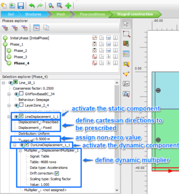
- the static (i.e., time-constant) component of a given prescribed displacement should be activated;
- the cartesian directions along which the displacement is to be prescribed should be defined;
- non-zero values should be assigned to the reference values of the prescribed cartesian components of the displacement, ux,start,ref and/or uy,start,ref (and/or uz,start,ref in PLAXIS 3D); please note that, when the dynamic component of the displacement is not activated, these reference values define a static displacement;
- the dynamic (i.e., time-dependent) component of the displacement should also be activated;
- a dynamic multiplier should be assigned to the prescribed cartesian components of the displacement; this multiplier may be defined in terms of displacement, velocity or acceleration; moreover, a non-zero value should be assigned to that scaling value of the dynamic multiplier.
These conditions are illustrated in the figure below for the case of a horizontal acceleration time-history (i.e., an earthquake motion) to be applied to the bottom boundary of a 2D model. It is important to note that:
- when the vertical acceleration time-history is to be disregarded, the displacement along the vertical direction should be restricted (i.e., Displacementy should be set to Fixed), to ensure equilibrium;
- the use of ux,start,ref= 0.5 m accounts for the fact that, in this particular case, an outcropping rock motion is being applied to the base of the model; please note that, as defined by the wave propagation theory, when a given body wave reaches a free surface, due to the impossibility of transmitting stresses, the amplitude of the motion is double from that of the incident wave; in addition, please note that, alternatively, it is possible to scale the amplitude of a given signal in the Multipliers window, by assigning a value different from 1.0 to (scaling) value.
- the units of the prescribed displacement (or velocity or acceleration) should be consistent with those defined in the Project properties.
Time evolution of a dynamic displacement
When a dynamic displacement is active in a given dynamic phase, the value of each of its components (e.g., along x-direction) at each instant of dynamic time, t, is given by:
ux(t) = ux,start,ref x multiplierx(t)
where ux,start,ref is the reference value of the static component of the prescribed displacement and multiplierx(t) is the time-dependent multiplier of the prescribed displacement.
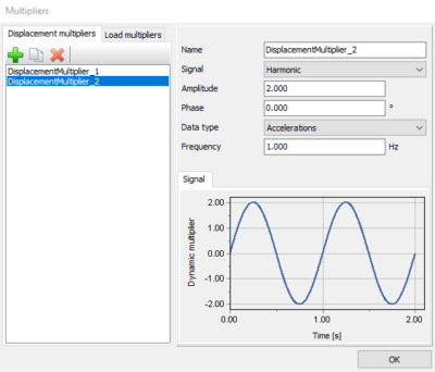
For instance, assuming that, in a 2D analysis, a given x-component of a dynamic displacement would be defined by a reference value, ux,start,ref, of 0.5 m, as well as by a harmonic multiplier defined in terms of accelerations and characterised by an amplitude of 2.0 m/s2, a frequency of 1.0 Hz and a null phase (as shown in the figure below), the dynamic motion applied to the model at 0.25 s would be equal to:
ax (t = 0.25 s) = -0.5 x 2.0 x sin(2 p x 0.25) = -0.5 x 2.0 = -1.0 m/s2.
Supposing now that two consecutive dynamic phases would be computed, the former having a dynamic time interval of 0.25 s, while the latter having a dynamic time interval of 0.75 s, and that time would not be reset at the start of the second dynamic phase, the first quarter of cycle of the sinusoidal motion (i.e., from 0 to 0.25 s) would be applied to the model during the first phase, while the remaining part of the first cycle (i.e., from 0.25 to 1.0 s) would be applied to the model during the second phase. Please note that the same principle applies when a given dynamic signal is defined by a table of values, rather than by a harmonic function.
Source: Bentley Communities
Categories
Finite Element / Finite Difference
Keywords
PLAXIS, PLAXIS2D
Form
Looking for more information? Fill in the form and we will contact Bentley Systems for you. Alternatively, you can visit Bentley's website and speak with a Bentley Geotechnical Expert.